In KWANT, there is a built-in function to plot band structure for the infinite system (or bulk system). Wraparound method in KWANT can draw the band structure of the bulk system in 3D plot. Then how to plot band structures along k-path in reciprocal space? Unfortunately, there are no built-in functions to plot band structures along the k-path. So, I will show you how to draw that by using KWANT.
As an example, let's suppose that we want to draw a band structure of monolayer graphene and bilayer graphene.
(1) Defining the system
import kwant
import numpy as np
import scipy.sparse.linalg as sla
import scipy.linalg as la
import tinyarray as ta
from numpy import sqrt

lat_const = 0.246  # lattice constant of graphene (unit: nm)
t         = 3.0    # nearest neighbor hopping parameter for graphene (unit: eV)
tn        = 0.3    # interlayer hopping between graphene (unit: eV)

def make_system(type_graphene = 'monolayer'):

    Bravais_vector = [(    lat_const,                     0),
                      (0.5*lat_const, 0.5*lat_const*sqrt(3))] # Bravais vectors
    Bottom_Lat_pos = [(0, lat_const/sqrt(3)), (0,  0)]        # The position of sublattice atoms in Bottom layer
    Upper_Lat_pos  = [(0, 0), (0, - lat_const/sqrt(3))]       # The position of sublattice atoms in Upper layer

    Bottom_lat = kwant.lattice.general(Bravais_vector, Bottom_Lat_pos, norbs=1)
    B_sub_a, B_sub_b = Bottom_lat.sublattices

    if type_graphene == 'bilayer':
        Upper_lat  = kwant.lattice.general(Bravais_vector, Upper_Lat_pos , norbs=1)
        U_sub_a, U_sub_b = Upper_lat.sublattices

    sym = kwant.TranslationalSymmetry(Bravais_vector[0], Bravais_vector[1])
    bulk = kwant.Builder(sym)

	# define hopping and on-site potential on bottom layer graphene
    bulk[B_sub_a(0,0)] = 0
    bulk[B_sub_b(0,0)] = 0
    bulk[kwant.builder.HoppingKind((0,0), B_sub_a,B_sub_b)] = t
    bulk[kwant.builder.HoppingKind((0,-1),B_sub_a,B_sub_b)] = t
    bulk[kwant.builder.HoppingKind((1,-1),B_sub_a,B_sub_b)] = t

	# define hopping and on-site potential on upper layer graphene
    if type_graphene == 'bilayer':
        bulk[U_sub_a(0,0)] = 0
        bulk[U_sub_b(0,0)] = 0
        bulk[kwant.builder.HoppingKind((0,0), U_sub_a,U_sub_b)] = t
        bulk[kwant.builder.HoppingKind((0,-1),U_sub_a,U_sub_b)] = t
        bulk[kwant.builder.HoppingKind((1,-1),U_sub_a,U_sub_b)] = t
        bulk[kwant.builder.HoppingKind((0,0), U_sub_a,B_sub_b)] = tn

    return bulk
※ Notice that because we define 2D infinite system (bulk), the translational symmetry(sym) applying to the system has two directions.
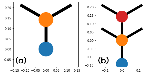
Then, the position of sub-atoms and their hopping in the unit cell for the monolayer and the bilayer graphene are as bellow;
monolayer_graphene = make_system(type_graphene="monolayer")
bilayer_graphene   = make_system(type_graphene="bilayer")

kwant.plot(monolayer_graphene)
kwant.plot(bilayer_graphene)
(2) wraparound method
Before plotting a band structure along k-path, let's use wraparound.
If you want to know specific information for this method, please refer to the following reference.
- kwant.wraparound: kwant-project.org/doc/dev/reference/kwant.wraparound
- kwant.wraparound.wraparound : kwant-project.org/doc/latest/reference/generated/kwant.wraparound.wraparound
- kwant.wraparound.plot_2d_bands: kwant-project.org/doc/dev/reference/generated/kwant.wraparound.plot_2d_bands#kwant.wraparound.plot_2d_bands
monolayer_wrapped = kwant.wraparound.wraparound(monolayer_graphene).finalized()
bilayer_wrapped = kwant.wraparound.wraparound(bilayer_graphene).finalized()

kwant.wraparound.plot_2d_bands(monolayer_wrapped)
kwant.wraparound.plot_2d_bands(bilayer_wrapped)
(3) Plotting the band structure along k-path
To achieve our goal, we use the code of kwant.wraparound.plot_2d_bands(). This code mainly consists of two parts;
* You can see the code: gitlab.kwant-project.org/kwant/kwant/blob/016b964/kwant/wraparound.py#L307-460
• From given basis vectors, obtain the first Brillouin zone (or Voronoi diagram in reciprocal space).
• Solve the eigenvalue equations at given k values
We use all of this code but separately use that.
First, let's obtain the coordinates of the edge of the FBZ (first Brillouin zone)
def First_BZ(finalized_bulk):
    # columns of B are lattice vectors
    B = np.array(finalized_bulk._wrapped_symmetry.periods).T
    # columns of A are reciprocal lattice vectors
    A = np.linalg.pinv(B).T

    # Get lattice points that neighbor the origin, in basis of lattice vectors
    reduced_vecs, transf = kwant.linalg.lll.lll(A.T)
    neighbors = ta.dot(kwant.linalg.lll.voronoi(reduced_vecs), transf)
    lat_ndim, space_ndim = finalized_bulk._wrapped_symmetry.periods.shape

    # Add the origin to these points.
    klat_points = np.concatenate(([[0] * lat_ndim], neighbors))

    # Transform to cartesian coordinates and rescale.
    # Will be used in 'outside_bz' function, later on.
    klat_points = 2 * np.pi * np.dot(klat_points, A.T)

    # Calculate the Voronoi cell vertices
    vor = scipy.spatial.Voronoi(klat_points)
    around_origin = vor.point_region[0]
    bz_vertices = vor.vertices[vor.regions[around_origin]]
    return vor, bz_vertices
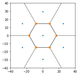
As return values, the coordinates of vertices of FBZ are received.
>>> vor, bz_vertices = First_BZ(wrapped)
>>> np.round(bz_vertices,2)
array([[ -8.51,  14.75],
       [-17.03,   0.  ],
       [ -8.51, -14.75],
       [  8.51, -14.75],
       [ 17.03,  -0.  ],
       [  8.51,  14.75]])
These vertices could be checked by using voronoi_plot_2d as bellow;
fig=scipy.spatial.voronoi_plot_2d(vor)
ax=fig.add_subplot()
plt.xlim(-40,40)
plt.ylim(-40,40)
ax.set_aspect('equal')
So, by using these points, we can write the high symmetric points and define their k-paths;
def symm_point(text:str):
    if    text == 'G': return np.array([0,0])
    elif  text == 'K': return bz_vertices[4]
    elif  text == 'M': return 0.5 * (bz_vertices[4] +bz_vertices[5])

def k_path(*args):
    dummy_1 = list(args[0])
    dummy_2 = dummy_1[1:]
    points = zip(dummy_1[:-1], dummy_2)

    k = []
    for p1, p2 in points:
        point1 = symm_point(p1)
        point2 = symm_point(p2)
        kx=np.linspace(point1[0],point2[0],50)
        ky=np.linspace(point1[1],point2[1],50)

        k.append(np.array(list(zip(kx,ky))))

    return np.concatenate(k)
Next, we solve the eigenvalue equations of Hamiltonian for given k values by using two functions in plot_2d_bands(), mommentum_to_lattice() and ham().
def momentum_to_lattice(syst, k):
    B = np.array(syst._wrapped_symmetry.periods).T
    A = np.linalg.pinv(B).T
    k, residuals = scipy.linalg.lstsq(A, k)[:2]
    if np.any(abs(residuals) > 1e-7):
        raise RuntimeError("Requested momentum doesn't correspond"
                               " to any lattice momentum.")
    return k

def ham(sys, k_x, k_y=None, **params):
    # transform into the basis of reciprocal lattice vectors
    k = momentum_to_lattice(sys, [k_x] if k_y is None else [k_x, k_y])
    p = dict(zip(sys._momentum_names, k), **params)
    return sys.hamiltonian_submatrix(params=p, sparse=False)
Then, let's define a function to calculate the band structure along k-paths;
def k_path_bandstructure(sys, *args):
    k_paths = k_path(args)
    energy = []
    for kx, ky in k_paths:
        energy.append(np.sort(np.real(np.linalg.eig(ham(sys, kx,ky))[0])))

    dummy  = np.linspace(0, len(args) - 1, len(energy))

    plt.figure(figsize=(10,5))
    plt.xticks(list(range(0,len(args))), list(args))
    plt.xlabel("k")
    plt.ylabel("energy [eV]")
    for n in range(len(args)):
        plt.axvline(x = list(range(0,len(args)))[n], color='black', linestyle = "--", linewidth = 1)
    for n in (np.array(energy)).T:
        plt.plot(dummy, n)
Then, the band structure of the monolayer and bilayer graphene along the following k-path (Gamma → K → M → Gamma) is as follows;
k_path_bandstructure(monolayer_wrapped, 'G', 'K', 'M','G')
k_path_bandstructure(bilayer_wrapped  , 'G', 'K', 'M','G')
In this way, we can draw the band structure for other materials
'소프트웨어 (계산용 프로그램) > Kwant' 카테고리의 다른 글
| [Kwant] Further-than-nearest-neighbor cells are connected by hopping (0) | 2021.02.09 |
|---|---|
| [Kwant-example] simple 1D chain (0) | 2020.04.03 |
| Ubuntu에서 Kwant 설치 (Anaconda) (2) | 2020.02.14 |
| Kwant에 대해서 (0) | 2020.02.14 |


댓글