Let's assume that we consider hoppings over the one unit cell. Then when you try to finalize the lead in KWANT, the message of "Further-than-nearest-neighbor cells are connected by hopping" occurs. Then, how do we solve this problem? There are two possible options to solve the problems [1];
(1) Extend translational symmetry of the lead
(2) Use wraparound method in KWANT
In order to illustrate two options, let's consider a simple case as follows;
As an example, a system with a hexagonal lattice is treated here. So, as a first step, let's define the system as below;
import kwant
import numpy as np

def make_system(length, width):
    def scattering_region(site):
        x, y = site
        return abs(x) <= 0.5 * length and abs(y) <= 0.5 * width

    ##########################################################################
    # Define the lattice structure
    ##########################################################################

    lat = kwant.lattice.honeycomb(a = 1)  # Honeycomb lattice
    bra = lat.prim_vecs                   # bra: the bravais vector
    sub_a, sub_b = lat.sublattices        # sublattice A and B of the hexagonal lattice
    sym = kwant.TranslationalSymmetry(bra[0])
    sym.add_site_family(lat.sublattices[0],other_vectors=[(-1,2)])
    sym.add_site_family(lat.sublattices[1],other_vectors=[(-1,2)])
    ##########################################################################
    # Define the scattering region and leads
    sys  = kwant.Builder()
    lead = kwant.Builder(sym)

    sys[sub_a.shape(scattering_region, (0,0))] = 0 # the onsite potential for sublattice A
    sys[sub_b.shape(scattering_region, (0,0))] = 0 # the onsite potential for sublattice B
    sys[lat.neighbors(1)] = 1                      # n.n hopping
    sys.eradicate_dangling()
    sys[lat.neighbors(2)] = 0.2                    # n.n.n hopping
    sys[lat.neighbors(3)] = 0.1                    # t.n.n hopping
    sys[lat.neighbors(4)] = 0.01                   # f.n.n hopping

    lead[sub_a.wire((0,0), 0.5 * width)] = 0 # the onsite potential for sublattice A
    lead[sub_b.wire((0,0), 0.5 * width)] = 0 # the onsite potential for sublattice B
    lead[lat.neighbors(1)] = 1               # n.n hopping
    lead.eradicate_dangling()
    lead[lat.neighbors(2)] = 0.2             # n.n.n hopping
    lead[lat.neighbors(3)] = 0.1             # t.n.n hopping
    lead[lat.neighbors(4)] = 0.01            # f.n.n hopping


    sys.attach_lead(lead)
    sys.attach_lead(lead.reversed())

    return sys, lead


sys, lead = make_system(3,3)
The plots of the system and a lead are;
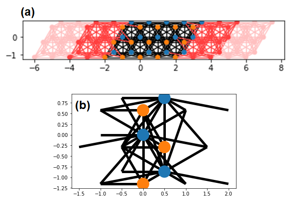
Note that the unit cell of leads (red color region) in fig (a) is different from that of a lead in fig. 1-(b). Before talking about this difference, let draw the energy dispersion of a lead in fig. 1-(b).
>>> kwant.plotter.bands(lead.finalized())

---------------------------------------------------------------------------
ValueError                                Traceback (most recent call last)
<ipython-input-60-827f0075f249> in <module>
----> 1 kwant.plotter.bands(lead.finalized())

/opt/anaconda3/lib/python3.8/site-packages/kwant/builder.py in finalized(self)
   1790             return FiniteSystem(self)
   1791         elif self.symmetry.num_directions == 1:
-> 1792             return InfiniteSystem(self)
   1793         else:
   1794             raise ValueError('Currently, only builders without or with a 1D '

/opt/anaconda3/lib/python3.8/site-packages/kwant/builder.py in __init__(self, builder, interface_order)
   2226                         msg = ('Further-than-nearest-neighbor cells '
   2227                                'are connected by hopping\n{0}.')
-> 2228                         raise ValueError(msg.format((tail, head)))
   2229                     continue
   2230                 if head_id >= cell_size:

ValueError: Further-than-nearest-neighbor cells are connected by hopping
(Site(kwant.lattice.Monatomic([[1.0, 0.0], [0.5, 0.8660254037844386]], [0.0, 0.0], '0', None), array([0, 0])), Site(kwant.lattice.Monatomic([[1.0, 0.0], [0.5, 0.8660254037844386]], [0.0, 0.5773502691896258], '1', None), array([-1, -1]))).
As you expected, the error message occurs. But, if we draw the lead's energy dispersion from "sys", the energy dispersion plot can be plotted properly.
>>> lead_1, _ = sys.leads
>>> kwant.plotter.bands(lead_1.finalized())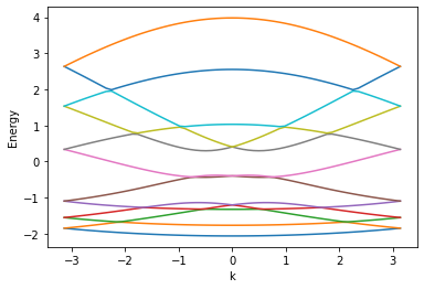
What happens here? Why does the energy dispersion of a lead cannot be obtained directly? Before discussing that, let's talk about the first way that I mentioned above.
1. Extend translational symmetry of the lead
The error message occurs because we treat hoppings that are longer range than 1 unit cell in Kwant. So, to resolve this problem, we extend the translational symmetry twice.
def make_system2(length, width):
    def scattering_region(site):
        x, y = site
        return abs(x) <= 0.5 * length and abs(y) <= 0.5 * width

    #################################################
    # Define the lattice structure of the graphene
    #################################################

    lat = kwant.lattice.honeycomb(a = 1)  # Honeycomb lattice
    bra = lat.prim_vecs                   # bra: the bravais vector of the graphene
    sub_a, sub_b = lat.sublattices        # sublattice A and B of the graphene
    sym = kwant.TranslationalSymmetry(2 * bra[0])
    sym.add_site_family(lat.sublattices[0],other_vectors=[(-1,2)])
    sym.add_site_family(lat.sublattices[1],other_vectors=[(-1,2)])
    #################################################
    # Define the scattering region and leads
    sys  = kwant.Builder()
    lead = kwant.Builder(sym)

    sys[sub_a.shape(scattering_region, (0,0))] = 0 # the onsite potential for sublattice A
    sys[sub_b.shape(scattering_region, (0,0))] = 0 # the onsite potential for sublattice B
    sys[lat.neighbors(1)] = 1                      # the nearest neighbor hopping
    sys.eradicate_dangling()
    sys[lat.neighbors(2)] = 0.2                    # the nearest neighbor hopping
    sys[lat.neighbors(3)] = 0.1                    # the nearest neighbor hopping
    sys[lat.neighbors(4)] = 0.01                   # the nearest neighbor hopping

    lead[sub_a.wire((0,0), 0.5 * width)] = 0 # the onsite potential for sublattice A
    lead[sub_b.wire((0,0), 0.5 * width)] = 0 # the onsite potential for sublattice B
    lead[lat.neighbors(1)] = 1               # the nearest neighbor hopping
    lead.eradicate_dangling()
    lead[lat.neighbors(2)] = 0.2             # the nearest neighbor hopping
    lead[lat.neighbors(3)] = 0.1             # the nearest neighbor hopping
    lead[lat.neighbors(4)] = 0.01             # the nearest neighbor hopping


    sys.attach_lead(lead)
    sys.attach_lead(lead.reversed())

    return sys, lead
Note that the translational symmetry of make_system2 is twice that of make_system.
Let draw the plot of the system and leads, and the energy dispersion of a lead as below;
>>> sys, lead = make_system2(3,3)
>>> kwant.plot(sys)
>>> kwant.plot(lead)
>>> kwant.plotter.bands(lead.finalized())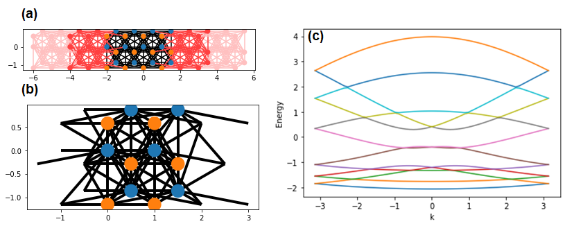
In contrast to the prior case we did, the energy dispersion from lead can be plotted and the error message doesn't occur. Also, the unit cell of the lead (Fig.3 (b)) is the same as that of sys (Fig.3 (a)).
I summarize the above results;
※ Summary
When there are hoppings whose range are over a unit cell in KWANT,
• The energy dispersion of leads cannot be obtained directly.
• But, if the lead is attached to the scattering system, its translational symmetry is automatically extended to cover all hoppings.
- For this reason, we could get the energy dispersion of a lead obtained from the system without an error message.
2. Use wraparound method in KWANT
The problem of the above way is the energy dispersion of the lead overlaps is overlapped in FBZ due to extended translational symmetry. This problem can be solved by wraparound method in KWANT. To illustrate it, we use systems that we defined before.
>>> sys, lead = make_system(3,10)The strategy is as follows;
(1) We apply the wraparound method to the lead ("lead") and finalize it.
(2) By using hamiltonian_submatrix, the Hamiltonian for k values is generated
(3) Solve the eigenvalue equation of the Hamiltonian
import scipy.linalg as la
import scipy.sparse.linalg as sla
import scipy
import numpy as np
from matplotlib import pyplot as plt
wrap_lead = kwant.wraparound.wraparound(lead).finalized()
energy_dispersion1 = []
kxrange = np.linspace( - np.pi, np.pi, 1000)
for kx in kxrange:
energy_dispersion1.append(np.linalg.eig(wrap_lead.hamiltonian_submatrix(params = dict(k_x = kx)))[0])
energy_dispersion1 = np.array(energy_dispersion1)
energy_dispersion1 = np.sort(np.real(energy_dispersion1))
plt.xlabel('k')
plt.ylabel('energy')
for n in range(len(energy_dispersion1.T)):
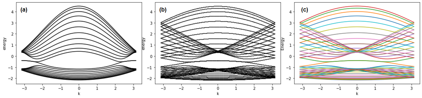
plt.plot(kxrange, energy_dispersion1.T[n],color='black')The made plot is as follows;

The plot is what we want. For width = 10, the plots made by the 1st way and the 2nd way are as follows. Note that Fig. 5 - (b) is obtained from the data of Fig. (a), which is generated by wraparound method. A "k" is extended twice and put into the first Brillouin zone. As you expect, the result is identical to the data made by the 1st way (extending translational symmetry).
Reference:
[1] www.mail-archive.com/kwant-discuss@kwant-project.org/msg01182.html
'소프트웨어 (계산용 프로그램) > Kwant' 카테고리의 다른 글
| [Kwant] Plotting the band structure along the k-path (8) | 2020.12.22 |
|---|---|
| [Kwant-example] simple 1D chain (0) | 2020.04.03 |
| Ubuntu에서 Kwant 설치 (Anaconda) (2) | 2020.02.14 |
| Kwant에 대해서 (0) | 2020.02.14 |


댓글